Grover's Search

Part of Womanium Quantum + AI 2024 program

Definition

Grover's search is unstructured quantum search algorithm that provides a clear quantum advantage over classical unstructured search.

Grover's search helps to speed up general functions with no other promises. (quadratic speed up)

Unstructured Search Example

Searching a function f:{0,1}^2 -> {0,1} to find x such that f(x) = 1

Classical approach is a linear search with a complexity of $O (2^{n})$
Quantum approach gives a complexity of $O (\sqrt{2^{n}})$

Grover's Algorithm

Grover's Algorithm works by repeating a specific process multiple times to ultimately increase the probability of measuring the "correct" answer. This process of increasing the probability of the right answer is known as amplitude amplification.

Grover's Algorithm makes use of a quantum oracle that can indicate the "correct" answer, which is the target of the search.

There are different ways to illustrate this algorithm, two of which are inversion around the mean and phase rotations.

Grover's Operator ( $\hat{G}$ )

\hat{G} = - H^{\otimes n} Z_{0} H^{\otimes n} Z_{f}

Where

$Z_{0}$ negates the phase if $| x ⟩$ is the all 0 string.

Z_{0} | x ⟩ = {\begin{cases} - | x ⟩ & x = 0^{\otimes n} \\ | x ⟩ & x \neq 0^{\otimes n} \end{cases} = (\begin{matrix} - 1 & 0 & \dots & 0 \\ 0 & 1 & \dots & 0 \\ ⋮ & ⋮ & ⋱ & ⋮ \\ 0 & 0 & \dots & 1 \end{matrix}) = I - 2 | 0^{n} ⟩ ⟨ 0^{n} |

This is basically an identity matrix where the first entry is -1.

$Z_{f}$ encodes oracle function $f$ , It's encoded using phase kickback such that the oracle’s results are stored in the phase. $Z_{f} | x ⟩ = (- 1)^{f (x)} | x ⟩$

Inversion Around the Mean

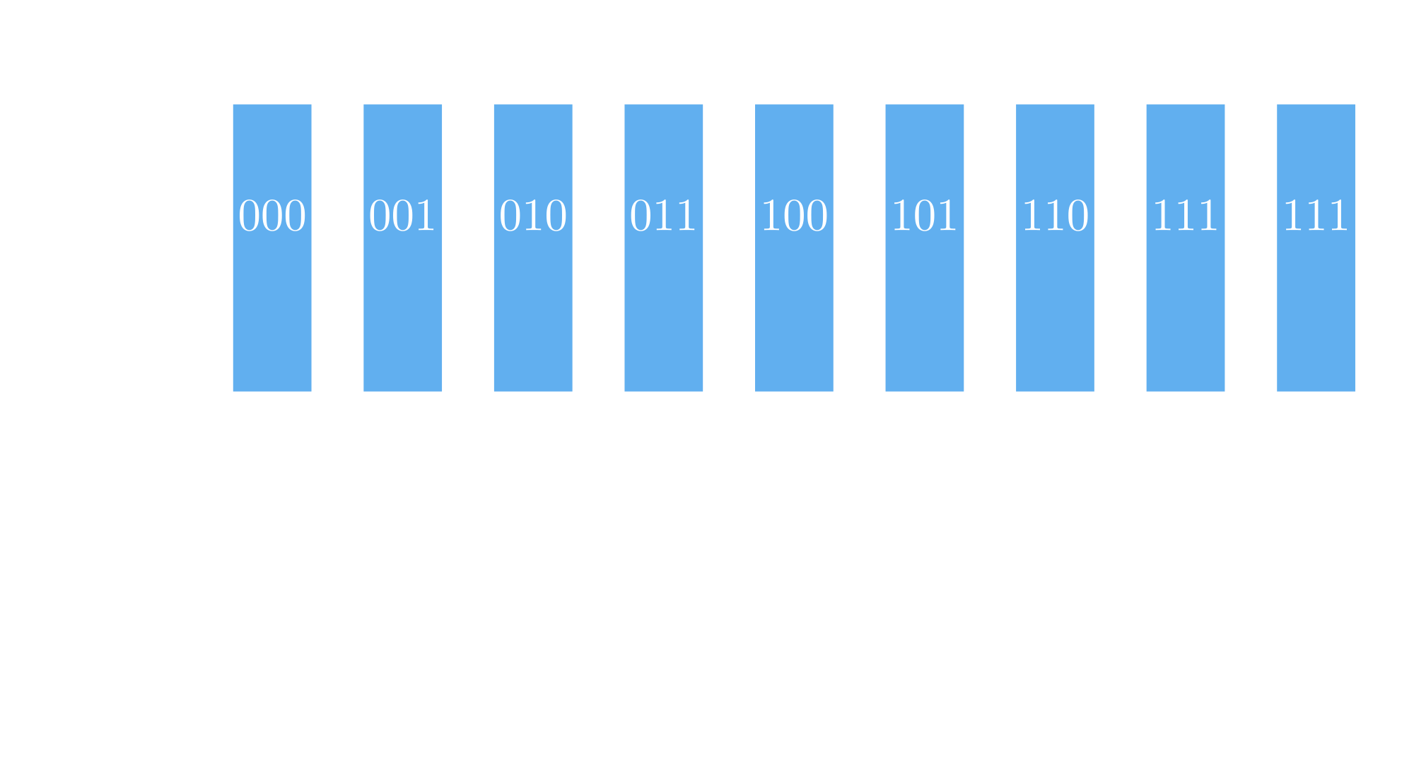
Let’s assume we have 8 options, but only 1 option is correct.

The algorithm start by setting an equal probability of measurement to each options (i.e. uniform superposition).

G1.png|700

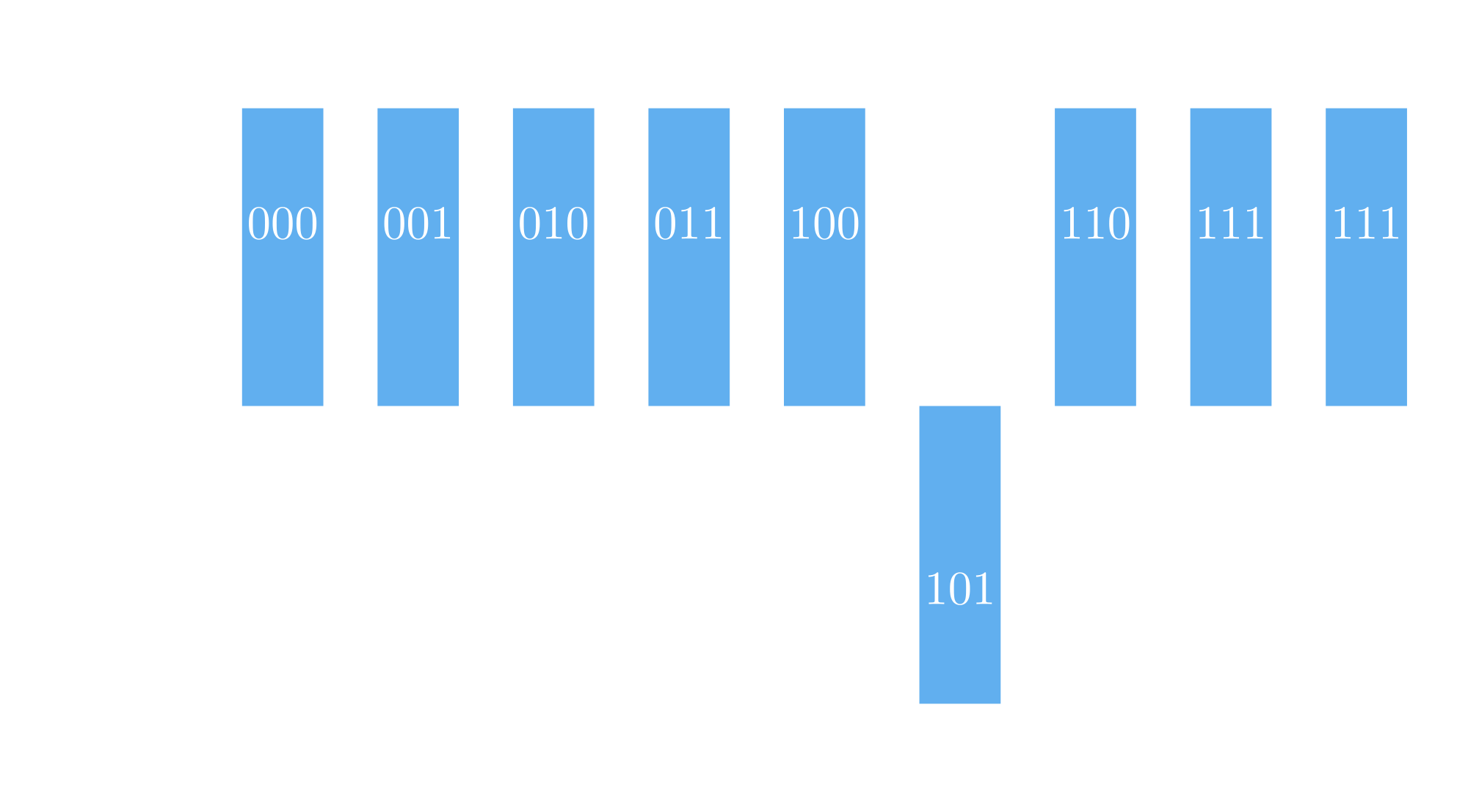
Then the oracle is queried, by doing that, the oracle "stores" the answer in the phase of the correct option, in other words it flips the phase of the correct option.

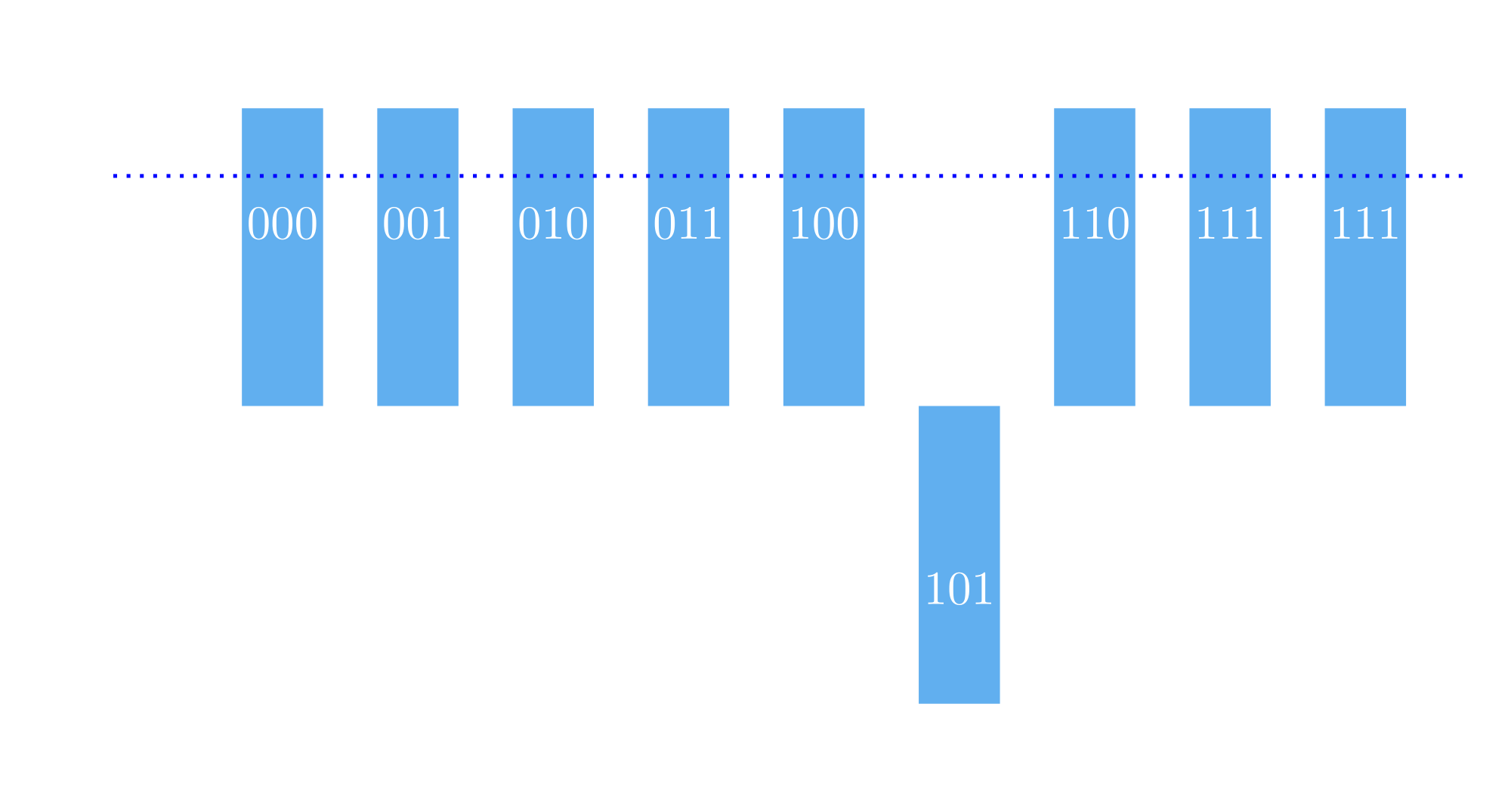
Now we apply Grover's operator ( $\hat{G}$ ), which computes the following for each option:

2 μ - α_{x}

Where:

$μ$ is the mean of the amplitudes.
$α_{x}$ is the amplitude of option $x$ .

The Grover's operator is defined in unitary operators as:

\hat{G} = - H^{\otimes n} Z_{0} H^{\otimes n} Z_{f}

grover's operator circuit.png

The $| 1 ⟩$ qubit is needed to enable the oracle to apply phase kickback.

This will lower the amplitude of all options except the option with an inverted phase, i.e. the correct answer.

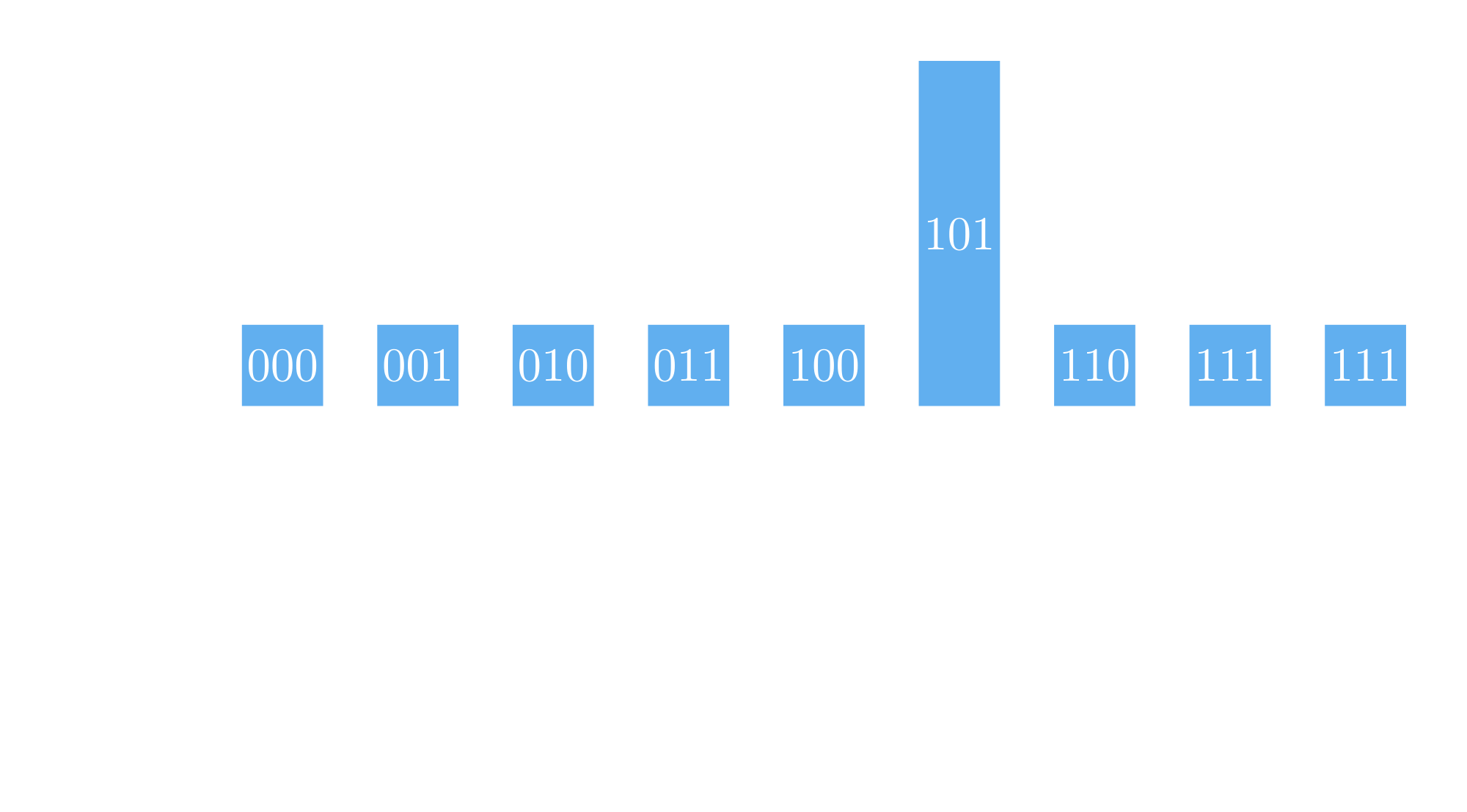
The figure clearly shows the amplification effect of the algorithm.

Finally, we repeat $\hat{G}$ for $k$ times, making sure not to overshoot the correct answer, since the mean might eventually get negative and destruct the amplitude of the correct answer.

Important

It's important to note that we are not exploring all options at once, as most people think, instead we manipulating the probability of measuring a specific result.

We are starting the algorithm with a superposition of all possible options, therefore it's only one quantum state and not multiple.

Applying Grover's Operator

To able to see how Grover's operator ( $\hat{G}$ ) applies our goal of inverting around the mean through $2 μ - α_{x}$ , we will re-express $\hat{G}$ as:

\hat{G} = - H^{\otimes n} Z_{0} H^{\otimes n} Z_{f} = U Z_{f}

such that

\begin{aligned} U & = - H^{\otimes n} Z_{0} H^{\otimes n} \\ = - H^{\otimes n} (I - 2 | 0^{n} ⟩ ⟨ 0^{n} |) H^{\otimes n} \\ = - (H^{\otimes n} - 2 H^{\otimes n} | 0^{n} ⟩ ⟨ 0^{n} |) H^{\otimes n} \\ = - (H^{\otimes n} - 2 | h ⟩ ⟨ 0^{n} |) H^{\otimes n} \\ = - (I - 2 | h ⟩ ⟨ 0^{n} | H^{\otimes n}) \\ = - (I - 2 | h ⟩ ⟨ h |) \\ = 2 | h ⟩ ⟨ h | - I \end{aligned}

$U$ is known as the diﬀusion operator, and it inverts the amplitudes about $μ$ .

where we define $| h ⟩$ as the Hadamard applied to $n$ qubits in the $| 0 ⟩$ state:

| h ⟩ = N^{- 1 / 2} \sum_{x \in {0, 1}^{n}} | 𝑥 ⟩, where N = 2^{n}

Finally, we can represent $U$ as the matrix:

\begin{aligned} U & = 2 (\frac{1}{\sqrt{N}} (\begin{array}{c} 1 \\ ⋮ \\ 1 \end{array}) \frac{1}{\sqrt{N}} (\begin{array}{c} 1 & \dots & 1 \end{array})) - I \\ = \frac{2}{N} (\begin{array}{c} 1 \\ ⋮ \\ 1 \end{array}) (\begin{array}{c} 1 & \dots & 1 \end{array}) - I \\ = \frac{2}{N} (\begin{array}{c} 1 & \dots & 1 \\ ⋮ & ⋱ & ⋮ \\ 1 & \dots & 1 \end{array}) - I \end{aligned}

Now we plug in $U$ into the state $x$

\begin{aligned} U \sum_{x \in {0, 1}^{n}} α_{x} | x ⟩ & = \sum_{x \in {0, 1}^{n}} α_{x} U | x ⟩ \\ = \sum_{x \in {0, 1}^{n}} α_{x} (\frac{2}{N} (\begin{array}{c} 1 & \dots & 1 \\ ⋮ & ⋱ & ⋮ \\ 1 & \dots & 1 \end{array}) - I) | x ⟩ \\ = \sum_{x \in {0, 1}^{n}} (2 \frac{α_{x}}{N} (\begin{array}{c} 1 & \dots & 1 \\ ⋮ & ⋱ & ⋮ \\ 1 & \dots & 1 \end{array}) - α_{x}) | x ⟩ \end{aligned}

But we know that

\sum_{x \in {0, 1}^{n}} \frac{α_{x}}{N} (\begin{matrix} 1 & \dots & 1 \\ ⋮ & ⋱ & ⋮ \\ 1 & \dots & 1 \end{matrix}) = \frac{\sum_{x \in {0, 1}^{n}} α_{x}}{N}

is the sum of the amplitudes of all options divided by their number, which means it's the mean $μ$ .

\begin{aligned} U & = \sum_{x \in {0, 1}^{n}} (2 \frac{α_{x}}{N} (\begin{array}{c} 1 & \dots & 1 \\ ⋮ & ⋱ & ⋮ \\ 1 & \dots & 1 \end{array}) - α_{x} I) | x ⟩ \\ = \sum_{x \in {0, 1}^{n}} (2 μ - α_{x}) | x ⟩ \end{aligned}

The final step to complete $\hat{G}$ is to plug in $Z_{f}$ :

\hat{G} = \sum_{x \in {0, 1}^{n}} (2 μ - α_{x}) Z_{f} | x ⟩ = \sum_{x \in {0, 1}^{n}} (2 μ - α_{x}) (- 1)^{f (x)} | x ⟩

We can see now that $U$ is responsible for inverting the amplitude around the mean, and $Z_{f}$ flips the phase of the correct answer through phase kickback.

Phase Rotations

We start by splitting our set of options into two sets, set $A$ contains "good" strings (strings we are searching for), and set $B$ containing bad string.

We show that as:

\begin{aligned} A = {x \in {0, 1}^{n} | f (x) = 1} \\ B = {x \in {0, 1}^{n} | f (x) = 0} \\ where \\ a = | A | = number of good strings \\ b = | B | = number of bad strings \end{aligned}

Now we define these sets as state vectors

\begin{array}{r} | A ⟩ = \frac{1}{\sqrt{a}} \sum_{x \in A} | x ⟩ \\ | B ⟩ = \frac{1}{\sqrt{b}} \sum_{x \in B} | x ⟩ \end{array}

Note

The set $A$ and the set $B$ are orthogonal sets, since there is no element that's shared between them, in other words, they're disjoint.

The overall system state $Ψ$ becomes

\begin{aligned} | Ψ ⟩ = α | A ⟩ + β | B ⟩ \\ ∴ α^{2} + β^{2} = 1 \end{aligned}

Since now we need to apply our operations on $| A ⟩$ and $| B ⟩$ , then let's define $| h ⟩$ in these terms.

| h ⟩ = \sqrt{\frac{a}{N}} | A ⟩ + \sqrt{\frac{b}{N}} | B ⟩

Applying Grover's Operator

In phase rotations representation it's beneficial to change the grouping of the operator from what we did last time. We group the operator as follows:

\hat{G} = - H^{\otimes n} Z_{0} H^{\otimes n} Z_{f} = (H^{\otimes n} Z_{0} H^{\otimes n}) (- Z_{f})

We notice that the first part is similar to $U$ , in fact, it is $- U$ , so we simplify it as:

- (2 | h ⟩ ⟨ h | - I) = I - 2 | h ⟩ ⟨ h |

Now for $- Z_{f}$ , we know that $Z_{f}$ applies a minus sign to the correct strings, therefore it will always assign a minus sign to all strings in $A$ , so we can say

- Z_{f} | A ⟩ = - (-) | A ⟩ = | A ⟩

We also know that $Z_{f}$ will not apply the minus sign for any string in $B$ , so we can say

- Z_{f} | B ⟩ = - (+) | B ⟩ = - | B ⟩

Now, we start applying the operator to the system then expanding it out to the state vectors $| A ⟩$ and $| B ⟩$ .

\begin{array}{r} \hat{G} | Ψ ⟩ = α \hat{G} | A ⟩ + β \hat{G} | B ⟩ \end{array}

Now we can apply the operator to each state vector separately.

\begin{aligned} \hat{G} | A ⟩ & = (I - 2 | h ⟩ ⟨ h |) (- Z_{f}) | A ⟩ = (I - 2 | h ⟩ ⟨ h |) | A ⟩ \\ = | A ⟩ - 2 | h ⟩ ⟨ h | A ⟩ \\ but \\ ⟨ h | A ⟩ = (\sqrt{\frac{a}{N}} ⟨ A | + \sqrt{\frac{b}{N}} ⟨ B |) | A ⟩ \\ = \sqrt{\frac{a}{N}} ⟨ A | A ⟩ + \sqrt{\frac{b}{N}} ⟨ B | A ⟩ = \sqrt{\frac{a}{N}} * 1 + \sqrt{\frac{b}{N}} * 0 \\ = \sqrt{\frac{a}{N}} \end{aligned}

This makes sense because $⟨ h |$ has an equal amplitude for all options $(\frac{1}{\sqrt{N}})$ and $| A ⟩$ has 1s only for the set $A$ strings.

\begin{aligned} ∴ & = | A ⟩ - 2 | h ⟩ ⟨ h | A ⟩ = | A ⟩ - 2 | h ⟩ \sqrt{\frac{a}{N}} \\ = | A ⟩ - 2 (\sqrt{\frac{a}{N}} | A ⟩ + \sqrt{\frac{b}{N}} | B ⟩) \sqrt{\frac{a}{N}} \\ = | A ⟩ - 2 (\frac{a}{N} | A ⟩ + \frac{\sqrt{a b}}{N} | B ⟩) \\ = | A ⟩ - \frac{2 a}{N} | A ⟩ - \frac{2 \sqrt{a b}}{N} | B ⟩ \\ = (1 - \frac{2 a}{N}) | A ⟩ - \frac{2 \sqrt{a b}}{N} | B ⟩ \\ \hat{G} | A ⟩ & = (1 - \frac{2 a}{N}) | A ⟩ - \frac{2 \sqrt{a b}}{N} | B ⟩ \end{aligned}

Now we apply $\hat{G}$ to $| B ⟩$

\begin{aligned} \hat{G} | B ⟩ & = (I - 2 | h ⟩ ⟨ h |) (- Z_{f}) | B ⟩ = (I - 2 | h ⟩ ⟨ h |) (- 1) | B ⟩ \\ = (2 | h ⟩ ⟨ h | - I) | B ⟩ = 2 | h ⟩ ⟨ h | B ⟩ - | B ⟩ \\ = 2 | h ⟩ \sqrt{\frac{b}{N}} - | B ⟩ \\ = 2 (\sqrt{\frac{a}{N}} | A ⟩ + \sqrt{\frac{b}{N}} | B ⟩) \sqrt{\frac{b}{N}} - | B ⟩ \\ = \frac{2 \sqrt{a b}}{N} | A ⟩ + \frac{2 b}{N} | B ⟩ - | B ⟩ \\ = \frac{2 \sqrt{a b}}{N} | A ⟩ + (\frac{2 b}{N} - 1) | B ⟩ \\ \hat{G} | B ⟩ & = \frac{2 \sqrt{a b}}{N} | A ⟩ - (1 - \frac{2 b}{N}) | B ⟩ \end{aligned}

Finally, we get it all together to finish applying $\hat{G}$ to the state $| Ψ ⟩$ .

\begin{aligned} \hat{G} | Ψ ⟩ & = α \hat{G} | A ⟩ + β \hat{G} | B ⟩ \\ = α ((1 - \frac{2 a}{N}) | A ⟩ - \frac{2 \sqrt{a b}}{N} | B ⟩) + β (\frac{2 \sqrt{a b}}{N} | A ⟩ - (1 - \frac{2 b}{N}) | B ⟩) \end{aligned}

$\hat{G}$ as a Rotation Operator

Let's define $\hat{G}$ as a unitary matrix

\hat{G} = (\begin{matrix} - (1 - \frac{2 b}{N}) & - \frac{2 \sqrt{a b}}{N} \\ \frac{2 \sqrt{a b}}{N} & 1 - \frac{2 a}{N} \end{matrix})

We notice that we can rewrite this matrix as

\hat{G} = (\begin{matrix} - (1 - \frac{2 b}{N}) & - \frac{2 \sqrt{a b}}{N} \\ \frac{2 \sqrt{a b}}{N} & 1 - \frac{2 a}{N} \end{matrix}) = {(\begin{matrix} \sqrt{\frac{b}{N}} & - \sqrt{\frac{a}{N}} \\ \sqrt{\frac{a}{N}} & \sqrt{\frac{b}{N}} \end{matrix})}^{2}

which is similar to the rotation matrix in Euclidean space

R (θ) = (\begin{matrix} \cos θ & - \sin θ \\ \sin θ & \cos θ \end{matrix})

Therefore, we can represent $\hat{G}$ as a rotation matrix which means that we can say the following.

Grover's operator is two rotation operators in Euclidean space, where:

\begin{array}{r} \cos θ = \sqrt{\frac{b}{N}} \\ \sin θ = \sqrt{\frac{a}{N}} \end{array}

such that after $k$ applications of $\hat{G}$ the state of the system can be represented as

| Ψ ⟩ = \cos ((2 k + 1) θ) | B ⟩ + \sin ((2 k + 1) θ) | A ⟩

where the goal of the algorithm is to maximize $\sin ((2 k + 1) θ)$ , such that $\sin ((2 k + 1) θ) \to 1$ .

Here we draw one application of $\hat{G}$ on the unite circle where:

$| Ψ ⟩$ , in purple, is the starting state.
$O | Ψ ⟩$ , in orange, is the state after applying the oracle.
$\hat{G} | Ψ ⟩$ , in green, is the state after applying $\hat{G}$ .

Pasted image 20240701231210.png

Note

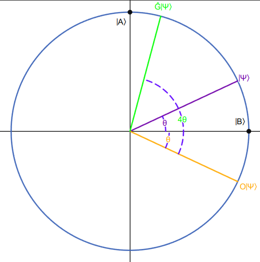
Notice that the starting state $| Ψ ⟩$ doesn't have to be in between $| A ⟩$ and $| B ⟩$ ( $θ = \frac{π}{4}$ ). The starting angle depends on the ratio of good and bad options $\frac{a}{b}$ .

Calculating $k$

Since out goal is to get $\sin ((2 k + 1) θ) \to 1$ , we can figure out $k$ as follows:

\begin{aligned} \sin ((2 k + 1) θ) \to 1 \\ ∴ (2 k + 1) θ \approx \frac{π}{2} \\ k \approx \frac{π}{4 θ} - \frac{1}{2} \\ but \\ \sin θ = \sqrt{\frac{a}{N}} \\ θ = \arcsin (\sqrt{\frac{a}{N}}) \\ θ \approx \sqrt{\frac{a}{N}} \end{aligned}

Important

Since the use of this algorithm only makes sense when we have a massive number of options to search through, we can assume that

\sqrt{\frac{a}{N}} \to 0

And therefore, we can approximate $\arcsin$ to be

\arcsin (\sqrt{\frac{a}{N}}) \approx \sqrt{\frac{a}{N}}

\begin{aligned} ∴ k & \approx \frac{π}{4 θ} - \frac{1}{2} \\ \approx \frac{π}{4 \sqrt{\frac{a}{N}}} - \frac{1}{2} \\ \approx \frac{π \sqrt{\frac{N}{a}}}{4} - \frac{1}{2} \\ k & \approx \frac{π \sqrt{\frac{N}{a}}}{4} - \frac{1}{2} \end{aligned}

Note

The computed value of $k$ is a lower bound of $k$ .

Complexity Analysis

We can assume that $\hat{G}$ is a constant-time operation ( $O (1)$ ), therefore we can define the time complexity by the number of iterations $k$ .

For the worst-case scenario we will assume $a = 1$ .

\begin{aligned} k & = \frac{π \sqrt{\frac{N}{1}}}{4} - \frac{1}{2} = \frac{π \sqrt{N}}{4} - \frac{1}{2} \\ ∴ O (k) & = O (\frac{π \sqrt{N}}{4} - \frac{1}{2}) \\ = O (\sqrt{N}) \end{aligned}

This proves that Grover's search algorithm offers a quadratic speed up over classical search of unstructured data.

Classical Search	Grover's Search
$O (N)$	$O (\sqrt{N})$

Circuit Implementation of the Diffusion Operator ( $U$ )

We discussed the application and effect of Grover's diffusion operator $U$ , but we didn't explore how it's implemented in a quantum circuit. Recall that

U = 2 | h ⟩ ⟨ h | - I

Let's see how we can implement that in a circuit. Note that we will be implementing $- U$ instead of $U$ , which will not effect the measurement results as long as we are consistent.

Now let's expand the form $- U$ to be able to construct the gates.

\begin{aligned} - U & = I - 2 | h ⟩ ⟨ h | = I - 2 (H^{\otimes n} | 0 ⟩ ⟨ 0 | H^{\otimes n}) \\ = H^{\otimes n} H^{\otimes n} - 2 H^{\otimes n} | 0 ⟩ ⟨ 0 | H^{\otimes n} \\ = H^{\otimes n} (H^{\otimes n} - 2 | 0 ⟩ ⟨ 0 | H^{\otimes n}) \\ = H^{\otimes n} (I - 2 | 0 ⟩ ⟨ 0 |) H^{\otimes n} \end{aligned}

We can see that we have two Hadamard operators at each end which we can simply implement with two Hadamard gates. Since we know how to implement the Hadamard operators, let's discard of them.

H^{\otimes n} (I - 2 | 0 ⟩ ⟨ 0 |) H^{\otimes n} \to I - 2 | 0 ⟩ ⟨ 0 |

But from constructing the diffusion operator earlier we know that the remaining part is just flipping the sign of the zero state $| 0 ⟩$ , which we can do with a Controlled-Z gate, but since we are looking for the zero-state and not the one-state we need to flip all the states before the Controlled-Z gate, then flip them back.

Finally, we can implement the diffusion operator as shown in the image:

U operator.png|700

Applying Multi-Controlled-Z Gate

Notice that we can apply the MCZ gate to an arbitrary target since it would result in the same effect of flipping the sign of the entire state.

We also notice that the target bit of the Z gate is not contributing to the control, and that's because it is indirectly controlling the application of the Z gate, since $Z | 0 ⟩ = | 0 ⟩$ and only $Z | 1 ⟩ = - | 1 ⟩$

Summary

Grover's algorithm employs the following steps:

Let $X$ be an n-qubit register, initialized to $| 0^{n} ⟩$ . Using $n$ Hadamard gates $(H^{\otimes n})$ , put $X$ in a uniform superposition:
$| 0^{n} ⟩ \overset{H^{\otimes n}}{\to} N^{- 1 / 2} \sum_{x \in {0, 1}^{n}} | 𝑥 ⟩ = | h ⟩$
Apply the unitary transformation $\hat{G} = - H^{\otimes n} Z_{0} H^{\otimes n} Z_{f}$ to register $X$ $k$ times.
Measure register $X$ and output result.

Grover's search algorithm offer a quadratic speed up over classical search (linear search) for unstructured data.

< Prev

Definition

Grover's Algorithm

Grover's Operator (G^)

Inversion Around the Mean

Applying Grover's Operator

Phase Rotations

Applying Grover's Operator

G^ as a Rotation Operator

Calculating k

Complexity Analysis

Circuit Implementation of the Diffusion Operator (U)

Summary

Grover's Operator ( $\hat{G}$ )

$\hat{G}$ as a Rotation Operator

Calculating $k$

Circuit Implementation of the Diffusion Operator ( $U$ )